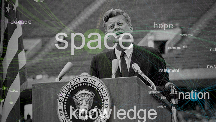
Interested in learning how to build a simple speech-to-text data pipeline in a few lines of code? Want to learn how to generate a beautiful data visualization to get insights into a speech or text? This article is for you.

I’ll walk thru how to build a speech recognition data pipeline using python and the Google Clouds speech-to-text API. We’ll touch on the basics of building a network graph from a text data source. And we’ll finish off by generating data visualizations using Gephi.

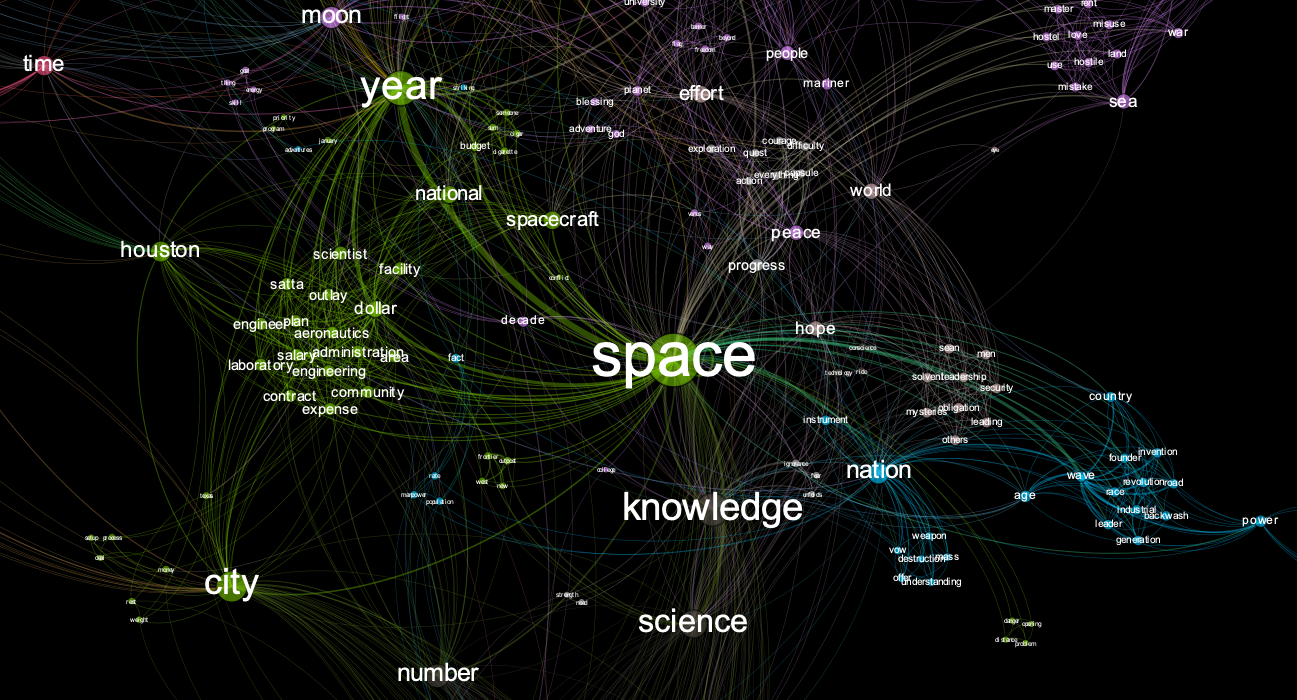
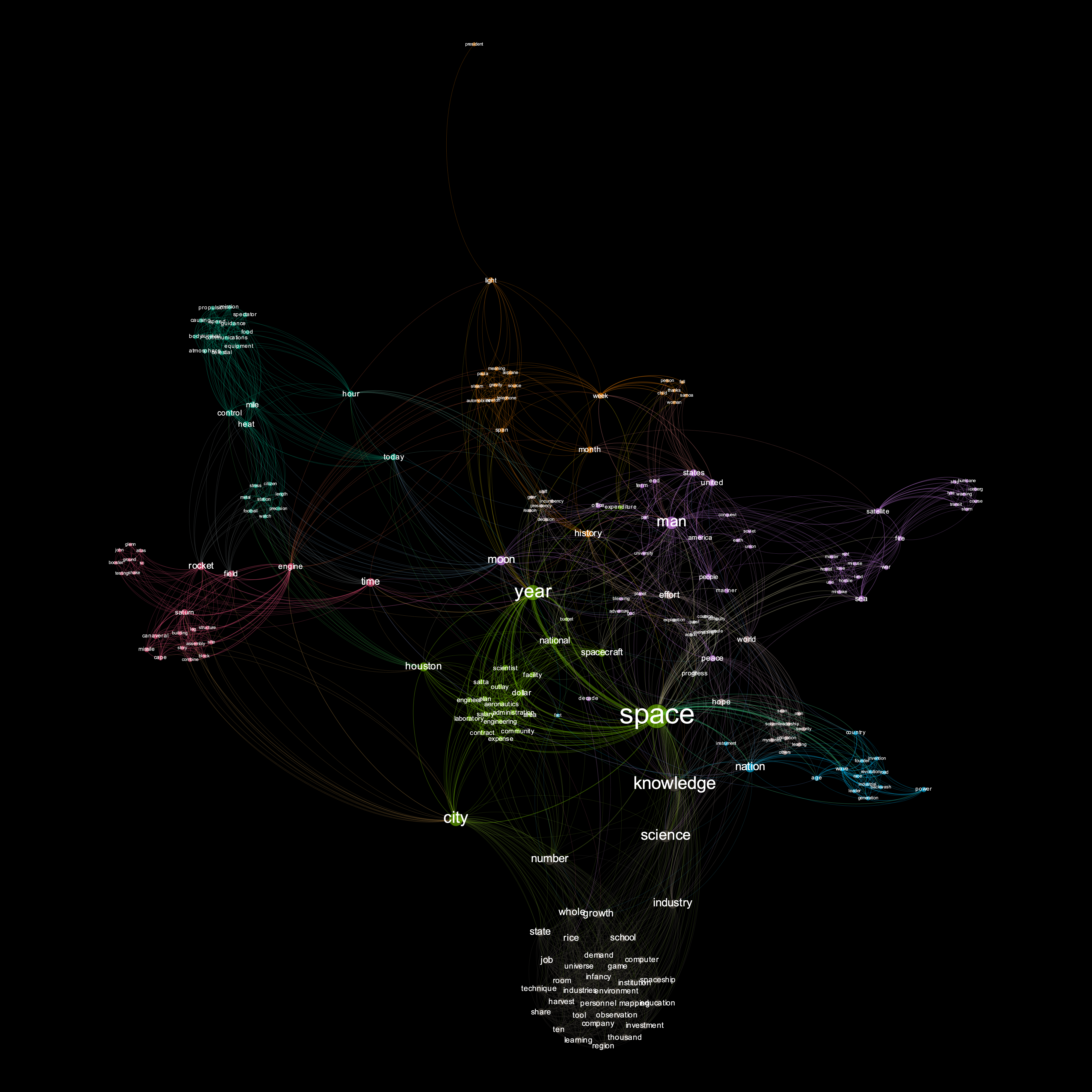
By the end of this article you’ll be able to generate neat graphs like the image below.

Backstory

After attending the 2019 Gartner Data & Analytics Summit, I was at the airport waiting for my flight back to SFO. I began wrangling my notes into something coherent I could share with my team back at the office.

I started with trying to outline the main themes of the keynote presentation. I had my notes, screen shots, and an mp3 audio file of the keynote speech. I didn’t want to listen to the entire keynote again, but my notes weren’t great. So I started playing with speech-to-text API’s to see if there was an easy way to transcribe the audio.

After getting the text transcribed, I still needed a way to extract key themes. I really liked the visualizations generated from texts at texttexture. So I started reading up on network graphs and how to produce network visualizations.

After a few hours I had a simple speech-to-text analytics pipeline working. It was a fun exercise and I was able to produce something neat to share with my team.

Hopefully this walkthru will save people time if they’ve got a similar use case.

Data Pipeline Overview

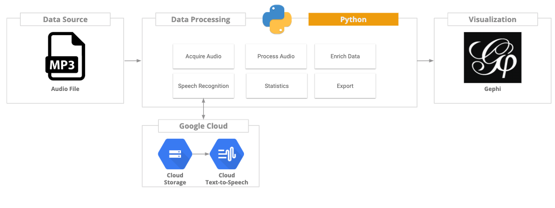
Here are the high level steps we’ll go thru to build out our data pipeline:

• Acquire the data. Extracting audio from a youtube video via the youtube API.
• Audio processing. Converting audio into wav format and converting to mono.
• Speech-to-text transcription. Using Google Cloud services, we’ll transcribe the audio speech into text.
• Data enrichment. Perform sentence and word tokenization. Text analytics. Data transformations.
• Graph model. Ingesting data into a network data model. Performing network transformations and statistics.
• Visualization. Viewing and creating a data visualization of our network model in Gephi.

Prerequisites

If you want to follow the steps in this article, you’ll need to install the following software on your machine:

• Jupyter Notebook
• Python 3.7.3
• Gephi 0.9.2
• Google Cloud
• Anaconda

Anaconda isn’t required. But it makes it easier to setup Jupyter and manage your python environment. Anaconda will have you up in running in no-time.

For reference, I tested this code on a Macbook Pro 2018 (i5) running MacOS Mojave 10.14.4.

Google Cloud

The speech transcription steps use the Google Cloud Speech-to-Text API. To access the API, you’ll need to sign-up for a google cloud developer account. The storage and Speech-to-Text API both offer free tiers. Make sure to watch your file size to stay in the free tier limits.

If you don’t want to sign-up for a google cloud account, you can use the streaming audio method via the public API key. The Ultimate Guide To Speech Recognition With Python article has a good write up on how to do that. The streaming method will get you up and running quick. But that method will not allow you to transcribe longer audio files longer than 1 min. But it can work with some mild data hi-jinx. If cutting audio into smaller sections and looping thru it via the streaming API doesn’t scare you go for it. That’s how I began playing around.

Required Python Packages

You’ll need to have the following list of python modules installed on your machine.

Pip installation of the packages should be straightforward.

pip install YOUR_PACKAGE_NAME

Google Cloud API

• gcloud==0.18.3
• google-api-core==1.9.0
• google-api-python-client==1.7.8
• google-auth==1.6.3
• google-auth-httplib2==0.0.3
• google-cloud==0.34.0
• google-cloud-core==0.29.1
• google-cloud-speech==1.0.0
• google-cloud-storage==1.15.0
• google-resumable-media==0.3.2
• googleapis-common-protos==1.5.9

Data Processing

• networkx==2.3
• nltk==3.4.1
• numpy==1.16.2
• python-louvain==0.13
• pandas==0.24.2

Audio Manipulation

• pydub==0.23.1

Youtube Download API

• youtube-dl==2019.4.30

Getting the Audio

The first step is to find an audio file that you wish to transcribe. For this article, we’ll use the JFK moon speech. I choose this audio source for a few reasons:

• The text transcript is available and can be used to cross check the speech to text output for accuracy
• The audio quality is not 100%, and I wanted to see how this would impact the text to speech transcription
• The speech had enough length and complexity to generate an neat data visual
• It’s an awesome speech!

If you already have an audio file you want to use, skip this step. Otherwise, for demo purposes you can use the code below to extract the audio from a youtube video to use as your audio source. The code block below will extract the audio portion of the requested video, and download it to your local machine in mp3 format.

Just replace the youtube URL with the video URL you wish to process.

from __future__ import unicode_literals
import youtube_dl

video_url='https://www.youtube.com/watch?v=ouRbkBAOGEw'

ydl_opts = {
    'format': 'bestaudio/best',
    'postprocessors': [{
        'key': 'FFmpegExtractAudio',
        'preferredcodec': 'mp3',
        'preferredquality': '192',
    }],
}
with youtube_dl.YoutubeDL(ydl_opts) as ydl:
    ydl.download([video_url])

[youtube] ouRbkBAOGEw: Downloading webpage
[youtube] ouRbkBAOGEw: Downloading video info webpage
[youtube] ouRbkBAOGEw: Downloading js player vflusCuE1


WARNING: unable to extract channel id; please report this issue on https://yt-dl.org/bug . Make sure you are using the latest version; see  https://yt-dl.org/update  on how to update. Be sure to call youtube-dl with the --verbose flag and include its complete output.


[download] Destination: JFK - We choose to go to the Moon, full length-ouRbkBAOGEw.m4a
[download] 100% of 16.18MiB in 00:0161MiB/s ETA 00:007
[ffmpeg] Correcting container in "JFK - We choose to go to the Moon, full length-ouRbkBAOGEw.m4a"
[ffmpeg] Destination: JFK - We choose to go to the Moon, full length-ouRbkBAOGEw.mp3
Deleting original file JFK - We choose to go to the Moon, full length-ouRbkBAOGEw.m4a (pass -k to keep)

Audio Processing - Prep Work

The next step is to prepare the audio file for text transcription. Our mp3 audio file needs to be converted into wav format and mono audio. We’ll use the pydub module for this.

import os
import pydub
from pydub import AudioSegment

directory_path = '/Users/jhuck/Documents/text_to_speech'
input_file_name = 'JFK - We choose to go to the Moon, full length-ouRbkBAOGEw.mp3'
output_file_name = 'JFK - We choose to go to the Moon, full length-ouRbkBAOGEw.wav'

#initialize our audio segment and set channels to mono
audio = AudioSegment.from_file(os.path.join(directory_path, input_file_name), format = 'mp3')
audio = audio.set_channels(1)

#export audio to wav format
audio.export(os.path.join(directory_path, output_file_name), format = 'wav')

<_io.BufferedRandom name='/Users/jhuck/Documents/text_to_speech/JFK - We choose to go to the Moon, full length-ouRbkBAOGEw.wav'>

Google Cloud Setup

Before accessing the Google APIs we need to do a bit of setup work to prep our local environment.

Storage Bucket

The Google Cloud Speech-to-Text API has two processing methods. For audio sources < 1 min in length, the streaming API can be used. For audio sources > 1 min length, the file needs to be loaded into a Google Cloud storage bucket before processing.

Setting up Google Cloud Storage only takes a few minutes. You’ll need to sign-up for a Google Cloud account if you don’t already have one. If you don’t already have a Storage bucket setup, create one now. Save the name of your storage bucket. You will need it to access the API and upload the audio file.

API Key

You need to generate an API key to access the Google Cloud API. The can be done via the Google Cloud Console. After you generate the key, download the API key JSON file to your local machine.

Enable the Speech-to-Text API

You’ll need to enable the speech to text API. Navigate to the Speech-to-Text API service and toggle the enable service switch.

Local Env Setup

Before accessing the Google Cloud API’s, you need to setup the credentials on your local environment. Local shell variable GOOGLE_APPLICATION_CREDENTIALS needs to be set. This can be done using the python commands below or via the terminal CLI.

import os
os.environ["GOOGLE_APPLICATION_CREDENTIALS"] = os.path.join(directory_path, 'My First Project-02d9aeddc2f8.json')

Upload File to Google Cloud

Now we’re ready to upload our audio file to Google Cloud using the Storage API. Alternatively you can load the file into the storage bucket using the Google Cloud Console GUI. Google has a lot of sample code snippets available for accessing the storage API.

from google.cloud import storage

def upload_blob(bucket_name, source_file_name, destination_blob_name):
    """Uploads a file to the bucket."""
    storage_client = storage.Client()
    bucket = storage_client.get_bucket(bucket_name)
    blob = bucket.blob(destination_blob_name)

    blob.upload_from_filename(source_file_name)

    print('File {} uploaded to {}.'.format(
        source_file_name,
        destination_blob_name))

gc_storage_bucket_name = your_storage_bucket_name

upload_blob(gc_storage_bucket_name ,os.path.join(directory_path, output_file_name) ,output_file_name)

File /Users/jhuck/Documents/text_to_speech/JFK - We choose to go to the Moon, full length-ouRbkBAOGEw.wav uploaded to JFK - We choose to go to the Moon, full length-ouRbkBAOGEw.wav.

Use Google Console to confirm the file has been uploaded.

Audio Transcription

At this point we’re ready to invoke the Speech-to-Text API and transcribe our audio file. The function below, transcribe_gcs, takes the URI of the file that we loaded to Google Cloud Storage an input. The file URI should be in format gs://YOUR_BUCKET_NAME/YOUR_FILE_NAME.

Timeout

I’ve hardcoded the timeout variable to 400 seconds. To productionalize this you’d want to setup a polling function to keep checking for results from the API call. If you get any errors due to timeout, try upping the timeout variable. For reference 400 seconds was long enough to transcribe 20 minutes of audio.

Punctuation

I’ve set the flag for punctuation to true. The API will attempt to add punctuation such as periods, commas, etc . We’ll use the punctuation during the text processing steps.

def transcribe_gcs(gcs_uri):
    """Asynchronously transcribes the audio file specified by the gcs_uri."""
    from google.cloud import speech
    from google.cloud.speech import enums
    from google.cloud.speech import types
    client = speech.SpeechClient()

    audio = types.RecognitionAudio(uri=gcs_uri)
    config = types.RecognitionConfig(
        encoding = enums.RecognitionConfig.AudioEncoding.LINEAR16,
        #sample_rate_hertz=16000,
        language_code='en-US',
        enable_automatic_punctuation=True)

    operation = client.long_running_recognize(config, audio)
    return_list = []
    print('Waiting for operation to complete...')
    response = operation.result(timeout=400)

    # Each result is for a consecutive portion of the audio. Iterate through
    # them to get the transcripts for the entire audio file.
    for result in response.results:
        #The first alternative is the most likely one for this portion.
        print(u'Transcript: {}'.format(result.alternatives[0].transcript))
        print('Confidence: {}'.format(result.alternatives[0].confidence))
        return_list.append(result.alternatives[0].transcript)
        
    return return_list

audio_file_uri = 'gs://' + gc_storage_bucket + '/' + output_file_name

output_text = transcribe_gcs(audio_file_uri)

Waiting for operation to complete...
Transcript: president Pizza vice president
Confidence: 0.8134621381759644
Transcript:  governor
Confidence: 0.8774576187133789
Transcript:  Congressman Thomas
Confidence: 0.9701719284057617
Transcript:  Senator while in Congress Mandela Bell
Confidence: 0.7495774626731873
Transcript:  sinus sting which gas at ladies and gentlemen, I appreciate you your president having made me an honorary visiting professor and I will assure you that my first light you will be a very brief. I am delighted to be here and I'm particularly delighted to be here on this occasion.

After you get the transcription text back, save it to a local file. You’ll notice that a confidence measure is provided for each text transcription. Overall, the Google API did a good job of transcribing the speech. But there are definitely mistakes comparing to the hand transcribed sources. This is probably due to the low quality audio source. The audio contains recording artifacts and noise that make transcribing the speech difficult.

The confidence measure could be used to identify and filter out low quality results. For our purposes, we’ll keep all of the audio transcription text the API generated.

output_text_file_name = 'jfk_moon.txt'

with open(os.path.join(directory_path, output_text_file_name), 'w') as f:
    for line in output_text:
        f.write("%s\n" % line.strip())

Text Processing

We’ve got our audio file transcription. It’s time to start processing the text. For this article, our end goal is to produce a network visualization of the text. To achieve this, we need to transform the text to fit a network model. Specifically, an undirected weighted graph.

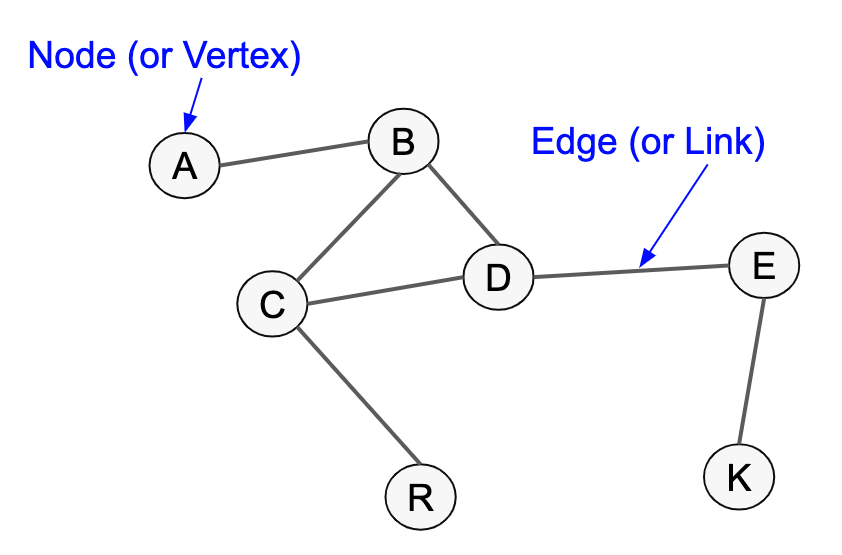
For our text, each word will become a node (or vertex). The relationship between the words will be the edges. Our final data output will be an array mapping the nodes and edges, including the weight (frequency).

For most of the text processing steps we’ll be leveraging the excellent natural language toolkit (nltk) module.

Sentence Tokenization

The next steps are about splitting the text into smaller chunks. We need to end up with individual words to map our nodes and edges.

Since we asked the Speech-to-Text API to add punctuation, there should be some level of punctuation available. We’ll search each transcribed string in our output text for periods. If a period is detected, we’ll use that to split the string into smaller tokens.

At the end of this step, we want a list that contains sentence like elements. For example, given the sentence “The fox jumped over the fence. And so did the lazy dog”. We’d want our array to contain two values: “The fox jumped over the fence”, “And so did the lazy dog”.

import nltk
from nltk.tokenize import sent_tokenize

#break out text into sentances
sentence_list = []

for line in output_text:
    if '.' not in line:
        sentence_list.append(line.strip())
    else:
        sent = sent_tokenize(line)
        for x in sent:
            sentence_list.append(x.strip())

Browse the output and sample the data to confirm that the text was tokenized correctly. The text transcription service will not add punctuation 100% correctly. So expect to see some incorrect sentence structures.

print(sentence_list[:10])

['president Pizza vice president', 'governor', 'Congressman Thomas', 'Senator while in Congress Mandela Bell', 'sinus sting which gas at ladies and gentlemen, I appreciate you your president having made me an honorary visiting professor and I will assure you that my first light you will be a very brief.', "I am delighted to be here and I'm particularly delighted to be here on this occasion.", 'We meet at a college.', 'noted for knowledge', 'They said he noted for progress in a state noted for strength and we stand in need of all three.', 'We meet in an hour of change and challenge.']

Word Tokenization

The next step is to further break down our sentences into individual words (tokens). Also, we want to add attribution to our words to identify the word class (noun, verb, punctuation, etc). Then we’re going to do a few data wrangling steps to cleanup and filter the data remove unwanted data points.

Stopwords

To extract the major themes from the text, we want to eliminate as much noise in the data as possible. One way to reduce noise is to filter out common “stopwords” like : a, for, so, etc . For our analysis, stop words will not add value and will be removed.

Alphanumerics

I’ve added in a step to filter out non-alphabetical (A-Z) characters. You can leave these in if you think your text has significant non-alpha elements of value.

Lemmatization

There’s also a step to perform text lemmatization to try and normalize the word set(ie. truck, trucks, truck’s = truck). More info on lemmatization found here.

Nouns

For this walk-thru, we’re only going to use nouns to build our text network. Nouns will help identify the major themes and simplify our word set.

Sentence Structure

For the later processing steps, we want to keep the sentence structure mapping. For example, we want to know if a word was in the first or second sentence. Our output from this step will be a 2D list in format: (sentence number, word)

from nltk import pos_tag, word_tokenize
from nltk.stem import WordNetLemmatizer
from nltk.corpus import stopwords
import re

word_list = []
word_exclude_list = []
lemmatizer = WordNetLemmatizer()

stop_words = set(stopwords.words('english'))
word_types = ['NOUN']
words_to_keep = ['united-states']

record_count = 0

for line in sentence_list:
    tokenized_text = nltk.word_tokenize(line)
    
    #tokenized text is array with format [word, word type]
    tagged_and_tokenized_text = nltk.pos_tag(tokenized_text,tagset='universal') 

    for token in tagged_and_tokenized_text:
        
        #For my use case i remove all non-alpha characters and lowered the text for uniformity. Modify for your use case
        token = [re.sub('[^a-zA-Z]+', '', token[0]).lower(),token[1]]
        
        if (token[1] in word_types and token[0] not in stop_words and len(token[0]) > 1) or token[0] in words_to_keep:
            word_list.append([record_count,lemmatizer.lemmatize(token[0])])

        else:
            word_exclude_list.append([record_count,token])
        
    record_count += 1

print(word_list[:10])

[[0, 'president'], [0, 'pizza'], [0, 'vice'], [0, 'president'], [1, 'governor'], [2, 'congressman'], [2, 'thomas'], [3, 'senator'], [3, 'congress'], [3, 'mandela']]

Undirected Graph

Now that we’ve got our list of words, it’s time to transform the data to fit our network model. Every element in our word list is going to serve as a node. The relationships between the nodes will form our edges.

Each individual word will serve as a node in our network. The edges between the nodes will be the word relationships within each sentence. To create the edge relationship, take each sentence and the associated set of words for that sentence. Then generate an unordered set without replacement for each word in the sentence.

For example, given set=(a,b,c), the output set would be:

• 1.(a,b)
• 2.(a,c)
• 3.(b,c)

Sentence example: “The sky is blue”

• 1.(the, sky)
• 2.(the, is)
• 3.(the, blue)
• 4.(sky, is)
• 5.(sky, blue)
• 6.(is, blue)

We’re going to use the itertools module to help with this step.

import itertools as it
import numpy as np

node_edge_list = []
node_list = []

record_count = 0

for word in word_list:
    sentence = ([row for row in word_list if record_count == row[0]])

    temp_list = []
    
    for token in sentence:
        temp_list.append(token[1])

    temp_cartesian_list = list(it.combinations(temp_list, 2))

    for i in temp_cartesian_list: 
        node_edge_list.append(i)
        
    record_count += 1

#Sort the list to make sure column 1 is always < column 2 regarding sort.
#Example, we don't want to count [(1,2), (2,1)]. We want [(1,2), (1,2)]
#This will impact the step when we aggregate the pairs to calculate the edge weights.
node_edge_list_array = np.array(node_edge_list)
node_edge_list_sorted_array = np.sort(node_edge_list_array, axis=1)
node_edge_list = node_edge_list_sorted_array.tolist()

temp_node_list = []

for i in node_edge_list:
    temp_node_list.append(i[0])

node_list = list(set(temp_node_list))

print(node_edge_list[:10])

[['pizza', 'president'], ['president', 'vice'], ['president', 'president'], ['pizza', 'vice'], ['pizza', 'president'], ['president', 'vice'], ['congressman', 'thomas'], ['congress', 'senator'], ['mandela', 'senator'], ['bell', 'senator']]

Edge Weights

To calculate the edge weights, you count the number of times that a pair of words appears in the array. Then aggregate the data to get the distinct node/edge combinations. SQL equivalent:

SELECT node
    , edge
    , COUNT(*) 
FROM word_array 
GROUP BY node, edge

We’re going to use pandas for this step. Aggregations are super easy using pandas data frames.

import pandas as pd

node_edge_dataframe = pd.DataFrame(node_edge_list,columns=['node', 'edge'])
node_edge_dataframe_count = node_edge_dataframe.groupby(['node','edge']).size().reset_index(name='counts')

output_edge_list_with_counts = node_edge_dataframe_count.values.tolist()

print(output_edge_list_with_counts[:10])

[['accelerator', 'automobile', 1], ['accelerator', 'equivalent', 1], ['accelerator', 'floor', 1], ['accelerator', 'power', 1], ['accuracy', 'canaveral', 1], ['accuracy', 'cape', 1], ['accuracy', 'line', 1], ['accuracy', 'missile', 1], ['accuracy', 'shot', 1], ['accuracy', 'stadium', 1]]

Create the Graph

At this point we’re ready to generate the network from our node/edge array. We’re going to use the networkx module to generate the network.

import networkx as nx

undirected_weighted_graph = nx.Graph()

for i in output_edge_list_with_counts:
    undirected_weighted_graph.add_edge(i[0], i[1], weight = i[2])
    
print(nx.info(undirected_weighted_graph))

Name: 
Type: Graph
Number of nodes: 347
Number of edges: 2706
Average degree:  15.5965

Graph Partitioning

To discover clusters or subgraphs within our network, we want to perform some type of graph partitioning to determine the node communities. This is a powerful step that will provide insights into the relationships that exist in our network.

For this article, I used the Louvain best community detection algorithm as it was straightforward to use and produced good results for my use case. After we execute the algo, we update our network with the partition results.

import community

graph_partition = community.best_partition(undirected_weighted_graph)
nx.set_node_attributes(undirected_weighted_graph, graph_partition, 'best_community')

Save the Model

We’re done wrangling data. Onto the visualization steps. Since we intend to use Gephi to visualize the data, we need export our dataset to disk in gexf file format.

output_file_name = 'network_output.gexf' 
nx.write_gexf(undirected_weighted_graph, os.path.join(directory_path, output_file_name))

Data Visualization

We’re ready to visualize our data. If you haven’t downloaded and installed Gephi, do it now.

Import GEXF File

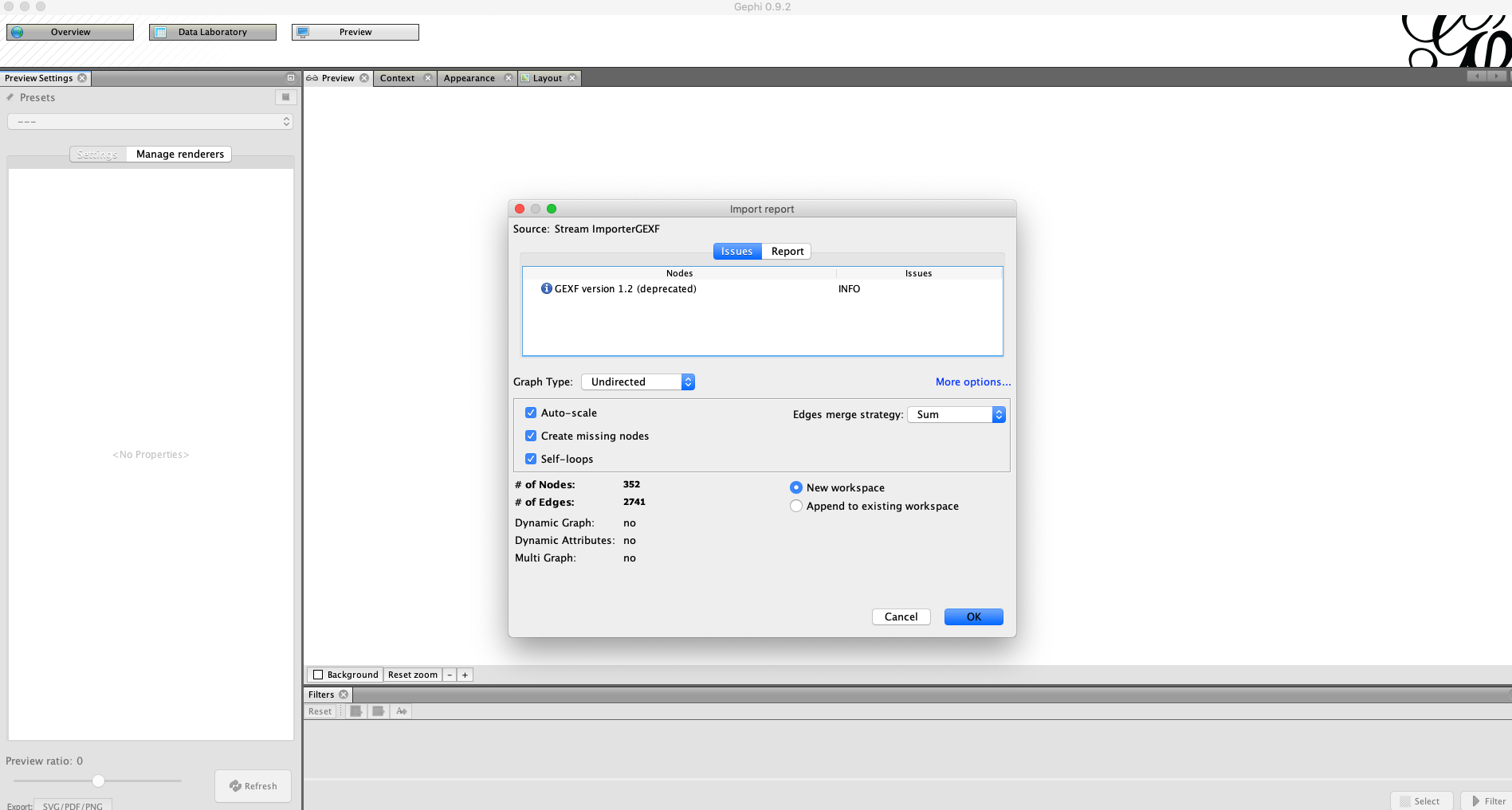
After you start Gephi, import the .gexf file we generated in the previous step.

Generate Preview

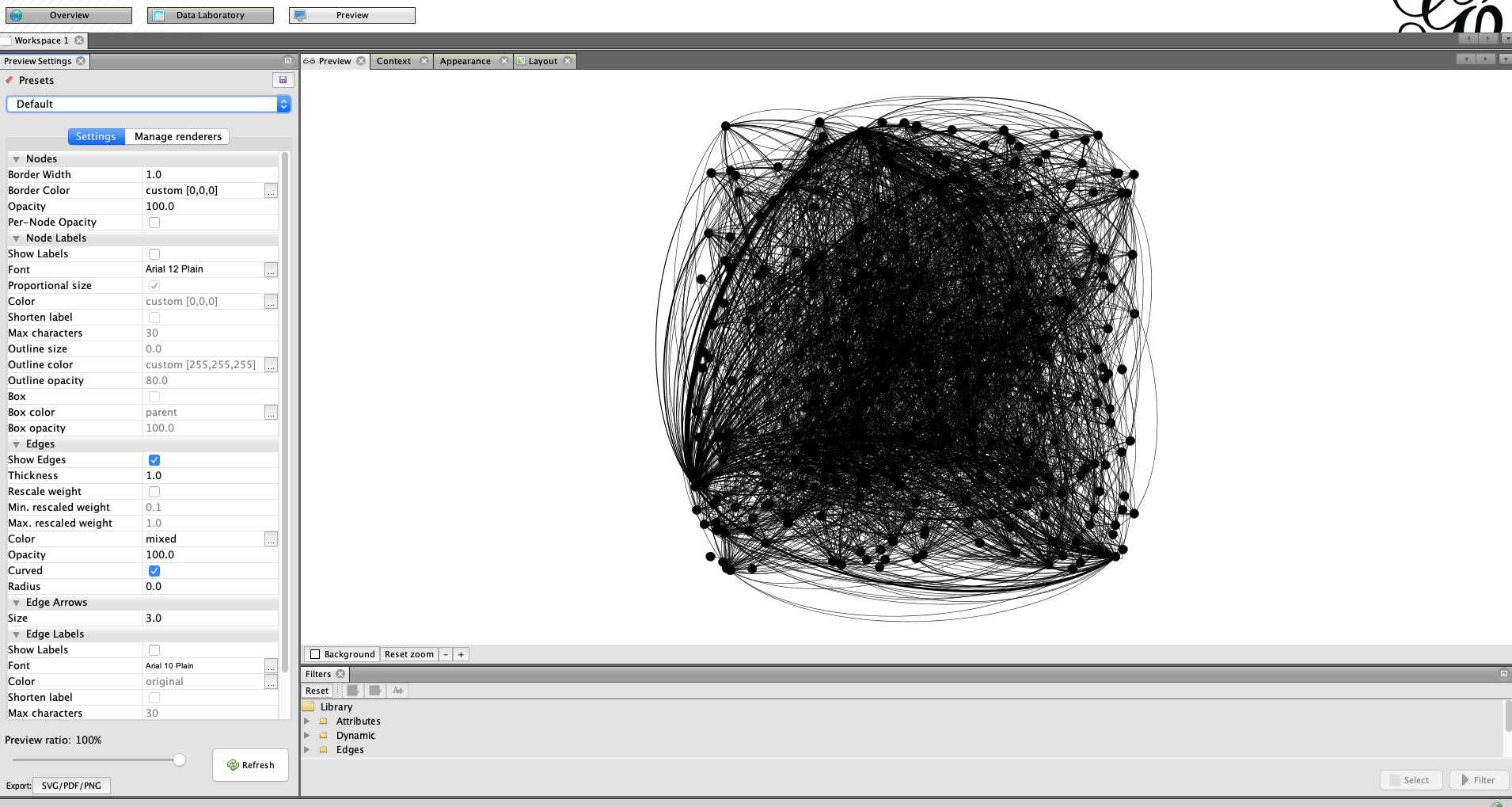
Go to the preview menu and run generate preview. At this point, you should see an incoherent jumble of black lines and dots.

Add Node Partitioning

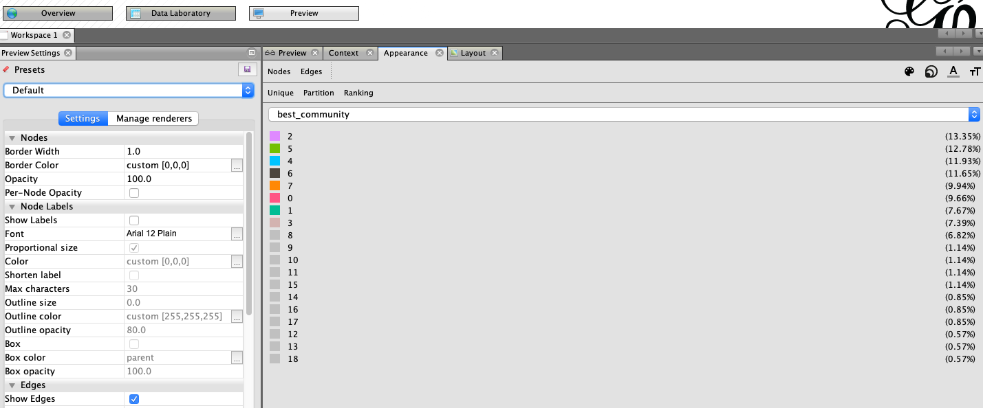
In the appearance menu, click on node, node size, then partition. Click the drop down and choose the best community attribute. This will modify the color of the nodes based on the best community partition we derived earlier.

Force Atlas Layout

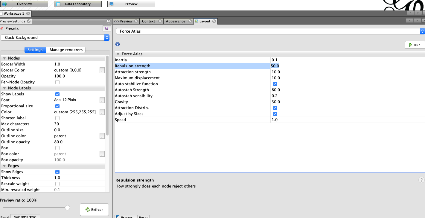
In the layout tab choose layout force atlas. Leave the default configurations. Hit run. You can stop it after a few seconds. This will rearrange the nodes based on the force layout algorithm. Feel free to play with the layouts or layout settings.

Change Preview Preset

Time to add some style. In the preview menu, change the style from default to black background. Feel free to use the default if you choose. The black layout looks cool though.

After your done, click preview again. You should now have a graph output similar to the image below.

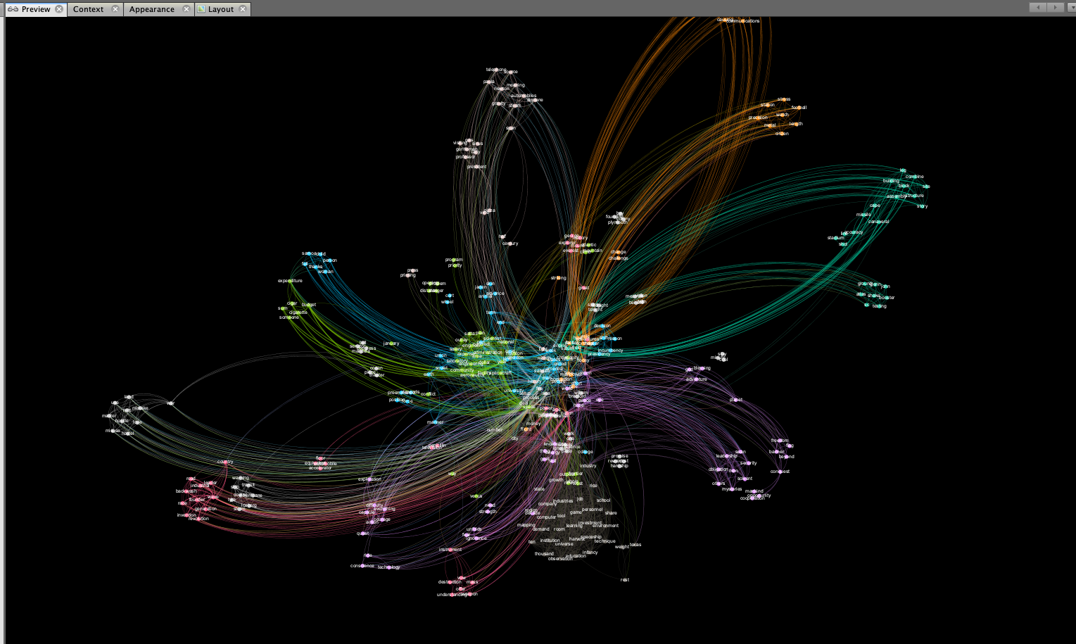
At this point you’ve got a cool looking network visualization. You can start digging in to find insights about the text. Try playing with the various filters to reduce noise. For large texts, filtering out nodes based on their degree or centrality can help to reduce graph clutter. For networks with a lage number of nodes, filters are your friend.

Wrap Up

This is the first time I’ve worked with Gephi and the Google Cloud speech-to-text API. Both were fun to use and it was a great learning exercise. I’ve run several texts and audio sources thru this process and gotten some cool results. Viewing text as a network diagram opens up new pathways for insights. Viewing text as a network graph makes it easy to visually identify key themes.

Speech driven apps like Alexa and Siri are continuing to grow in popularity. Demand for analytics pipelines involving audio as a data source will also ramp up. There’s a ton of potential for innovation in the space. Especially with streaming functionality. I’m excited to keep playing around with these tools.

For reference, here’s the full data viz image from the JFK moon speech.

You can access the code used in this post at my github repo located here.

References

Here’s a list of reference material I found helpful to get up to speed on speech-to-text, network graphs, text analytics, and Gephi.

• realpython.com/python-speech-recognition/
• analyticsvidhya.com/blog/2018/11/introduction-text-summarization-textrank-python/
• cloud.google.com/speech-to-text/docs/
• towardsdatascience.com/textrank-for-keyword-extraction-by-python-c0bae21bcec0
• analyticsvidhya.com/blog/2018/04/introduction-to-graph-theory-network-analysis-python-codes/
• harangdev.github.io/applied-data-science-with-python/applied-social-network-analysis-in-python/1/
• neo4j.com/docs/graph-algorithms/current/algorithms/louvain/
• textexture.com/
• JFK Photo by: Bob Gomel. Image overlayed with network visualization

Thanks for reading the post. Feel free to contact me with any feedback or questions.